Neural networks are long assumed to be a black box, and though that might still be true to an extent, it can be very helpful to try to understand what’s going on inside it. In this blog post, I’ll try to crack open this black box and present some very intuitive ways to interpret neural nets.
Knowing very surface-level linear algebra and neural network basics will make this post flow much easier. However, I try to not skip through any details. The video version of the blog post, which can be found here, assumes much less background.
This blog will be separated into three parts:
Visualizing Neural Networks In 2D
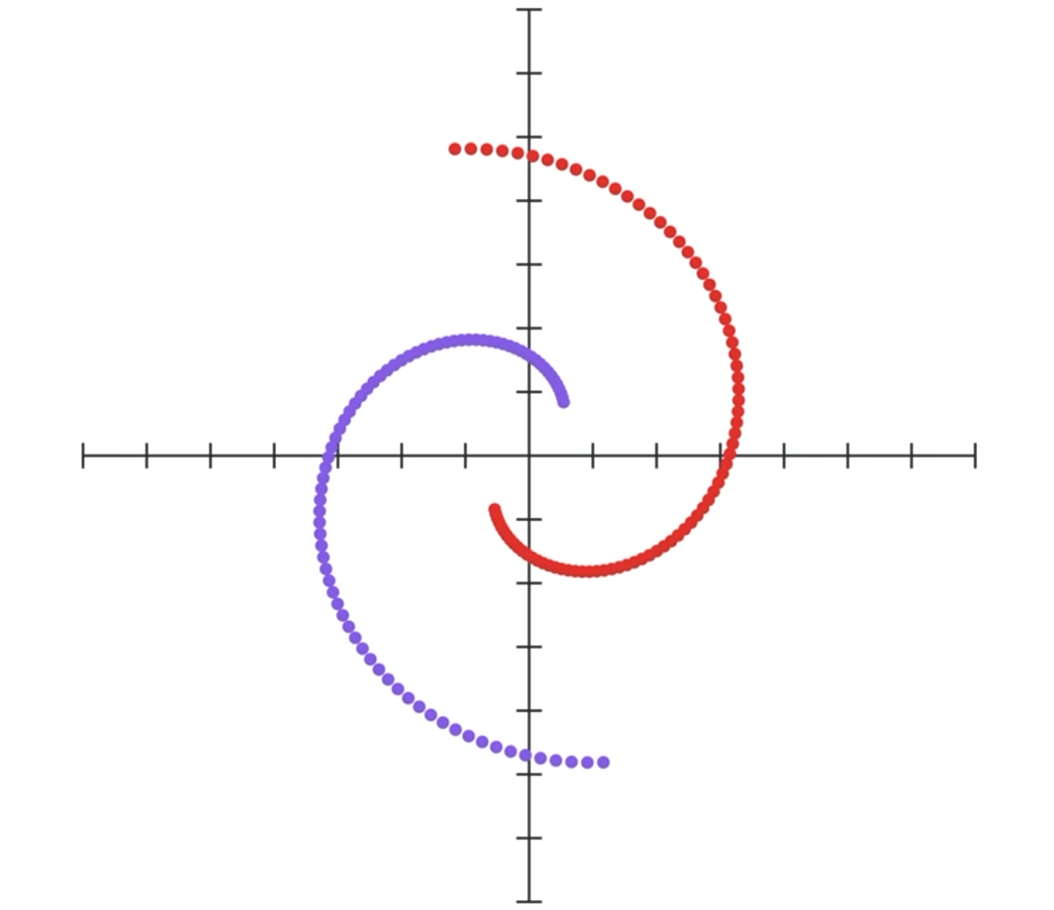
Let’s start with a simple example. Let’s say we have these two entangled spirals of different color, and our goal is to essentially separate them using a neural network.
Now I could just make a neural network that looks like this:
It takes as input the x and y coordinates of the dot, and outputs a value between 0 and 1, where a value closer to 0 means it’s purple, otherwise it’s red. The network will easily reach an error of 0, but our purpose here is to visualize what the network might be doing.
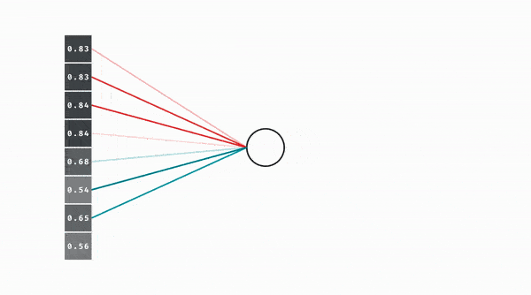
Let’s make our neural network one layer. Our input of 2 dimensions (x and y coordinates) will be mapped to a vector of 8 dimensions (since it has 8 neurons).
Unfortunately, our human brains aren’t capable of visualizing anything higher than 3 dimensions, so let’s bring down the neurons in the second layer to only 2.
This is much easier to visualize. We can now just treat that two dimensional vector that is output as x y coordinates. Or in other words, given a dot in our original 2D coordinate plane, that layer can be seen as just moving it to another place in the same coordinate plane.
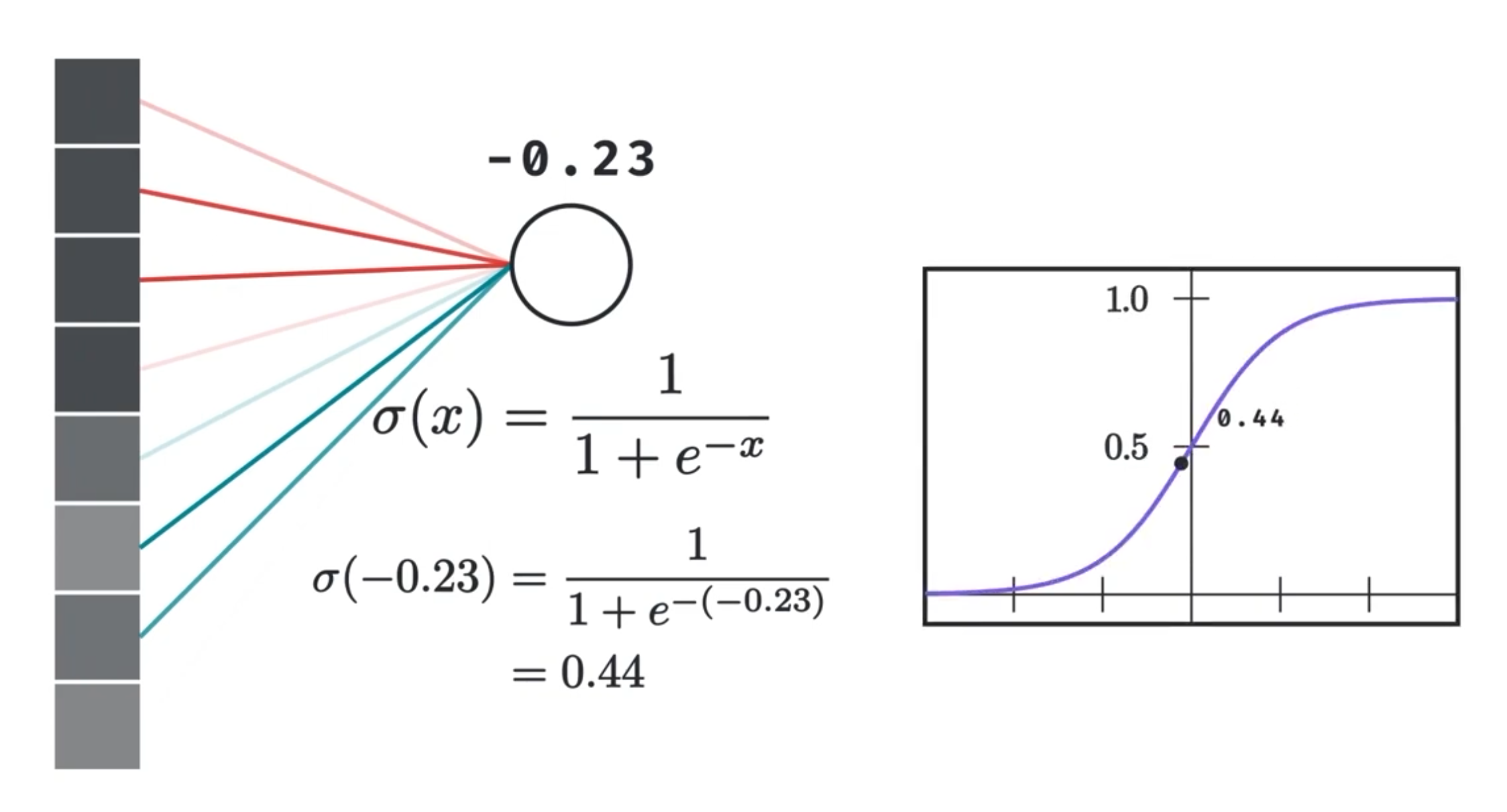
We know that a neuron in the second layer essentially represents a weighted sum between the weights and values of the previous layer’s neurons. That weighted sum is then passed to some other non-linear function like the sigmoid.
We do this for both the new x and y coordinates, and the whole thing becomes identical to mutiplying the original coordinate vector with a 2 by 2 matrix and then passing the result to a nonlinearity.
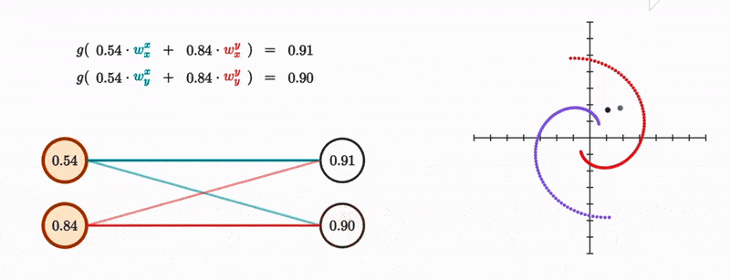
And this makes sense given that all the layer is doing is moving the dot linearily and then somehow nonlinearily, and if you know a bit of linear algebra, then you’ll know that matrix multiplication fundamentally represents a linear transformation to vectors. It’s also a useful visualization to see what this transformation does to the entire space at once as depicted from how it transforms the grid lines.
![]()
Our choice for non linearity from now on will be the tanh, which is defined as follows:
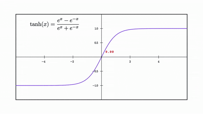
and as you can see it squishes our input into the range [-1 to 1].
Let’s look at what happens to our space when we apply a matrix multiplication followed by a tanh.
![]()
Here tanh is being applied to both the x and y coordinate. In other words, it’s applied element wise to our coordinate vectors, which is why both the x and y coordinates are squished to a range of -1 to 1.
In practice, we also add a constant we call the bias along with the weighted sum. This represents a translation. Here is a linear transformation followed by a translation followed by a tanh.
![]()
This now represents how a full layer would transform our input and space.
Note that a linear transformation followed by a translation is called an affine transformation, which is what we’ll call it from now on.
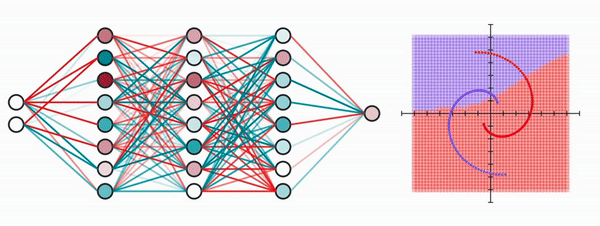
Going back to our spiral example, all we’re saying here is that a neural network layer is an affine transformation followed by a nonlinearity. If we make sure all our layers are only 2 neurons wide, then we can show the neural network as simply a series of those transformations in 2D!
So how would this look like for a fully trained neural network? Here’s the code I used to build the neural network using PyTorch, and you don’t need to understand the code, just that I used 5 fully connected layers each mapping from 2 neurons to 2 other neurons, and that I used the tanh as my choice of nonlinearity.
import torch
from torch import nn

class SpiralsClassifier2D(nn.Module):
    def __init__(self):
        super(SpiralsClassifier2D, self).__init__()
        # fully connected layers (FC)
        self.fc1 = nn.Linear(2, 2)
        self.fc2 = nn.Linear(2, 2)
        self.fc3 = nn.Linear(2, 2)
        self.fc4 = nn.Linear(2, 2)
        self.fc5 = nn.Linear(2, 2)

    def forward(self, input):
        x = torch.tanh(self.fc1(x))
        x = torch.tanh(self.fc2(x))
        x = torch.tanh(self.fc3(x))
        x = torch.tanh(self.fc4(x))
        return self.fc5(x)
This is how the network transforms our spiral dots!

You can see that our network is stretching and morphing our input in such a way as to cleanly separate the two types of dots.
At the end, once our dots are cleanly separated, we now simply draw a linear boundary separating the two classes. This is what the last layer is, which maps to a single number in this case. This can be thought of as projecting our data into a line such that the red dots are as negative as they can be and the blue dots are as positive as they can be. Or perhaps more intuitively with a bit of hand-waving, looking at this line’s perpendicular which gives us a nice linear boundary between the two classes.
To me, this is just beautiful. Behind all this complexity, this is the fundamental principle behind neural networks: affine transformations followed by nonlinear transformations.
Why Use More Neurons Per Layer?
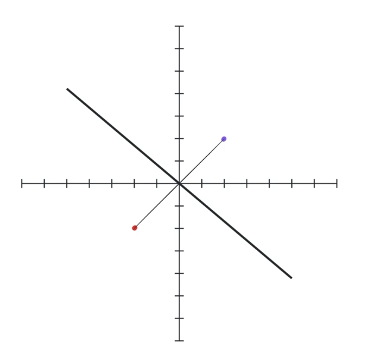
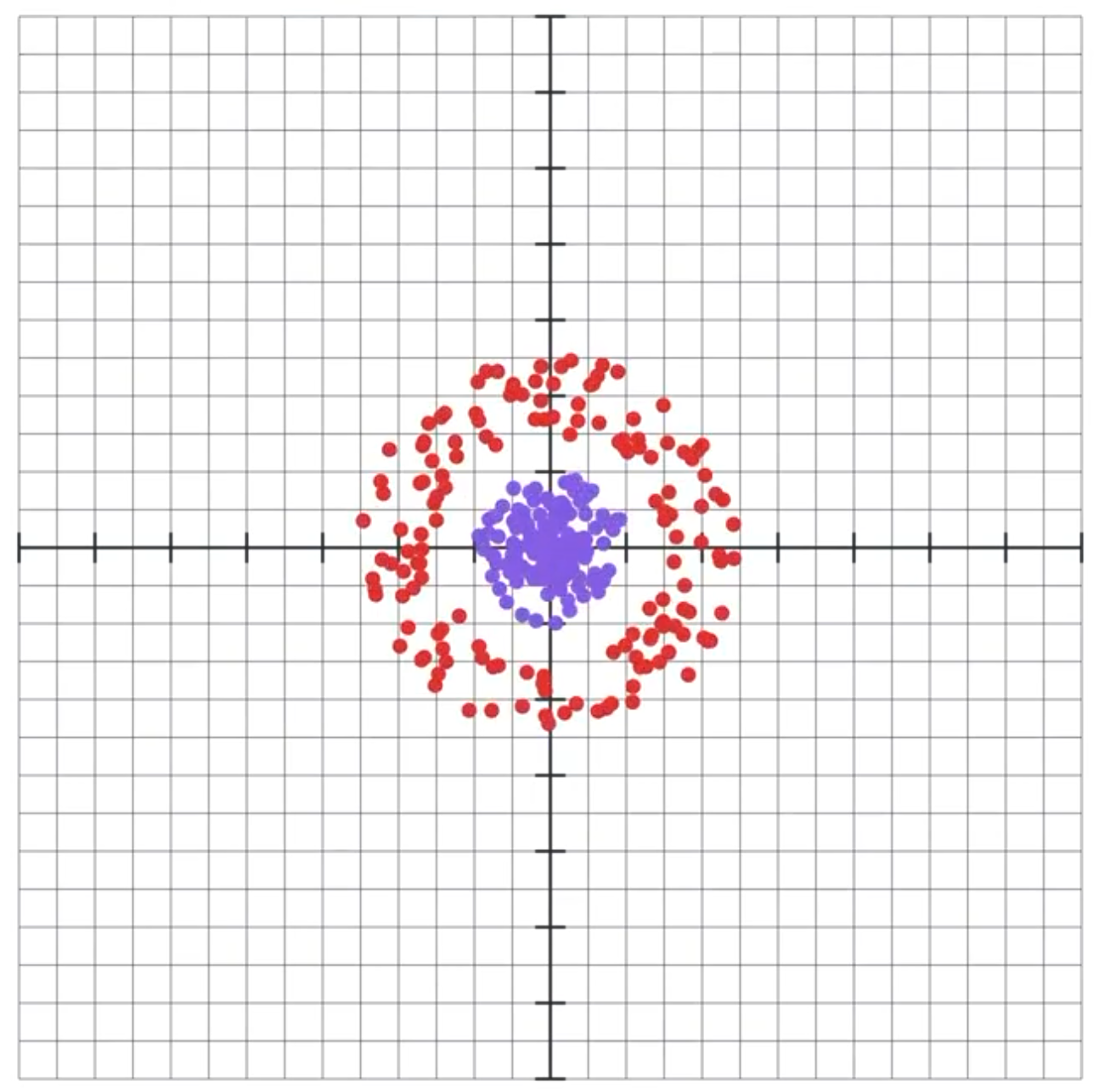
Now, using just two neurons is actually a huge limitation to our neural network. In fact, there are some boundaries that our network simply won’t be able to draw with just two neurons with a tanh activation no matter how many layers we add. Let’s look at this example where we want to separate the inner dots from the outer dots.
It’s possible to separate these using this specifically chosen nonlinear transformation (I actually used its inverse to generate the dots):
![]()
Now let’s try to see how our network of only two neurons per layer with a tanh activation will do as visualized by a sequence of transformation.

Let’s also look at it from another perspective, where we view some of the layers’ outputs in real time, and then show how those outputs evolve as the model trains.

Evidently, the model tries so hard to separate the two boundaries, but it just fails. Intuitively, you can think through what type of continuous morphing the model will have to do to separate the two colors, and that we simply can’t separate the two regions. Well, that is unless we tear the space somehow, but neither the affine transformation nor the tanh can do that. Besides, that would cause discontinuity problems and make training tricky.
But neural networks are universal approximators, so we already know that it can fit this boundary given enough neurons in one layer.
Here, and this is really cool, by just adding one more neuron and thus changing output spaces into 3 dimensional spaces, we get the following:
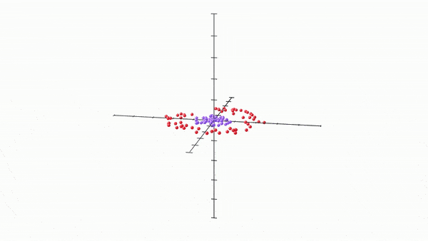
Once our model got access to the third dimension, i.e. got 3 neurons per layer, it very quickly found a way to separate the two regions by allowing the space to “bulge” out into the third dimension, and then the two regions simply become separable by a plane in the middle. It essentially got access to way more wiggle room to move around and separate.
I was struck in awe when I saw this for the first time. This essentially demonstrates to us, intuitively, the utility of using more neurons per hidden layer, i.e, increasing the dimensions of our hidden layers.
Manifold Hypothesis
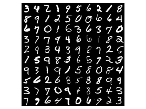
But how does this translate to real life datasets though? I mean, we won’t exactly get a dataset of, say, 28 by 28 handwritten digits images, where the images will form a structured shape within the input space, right?
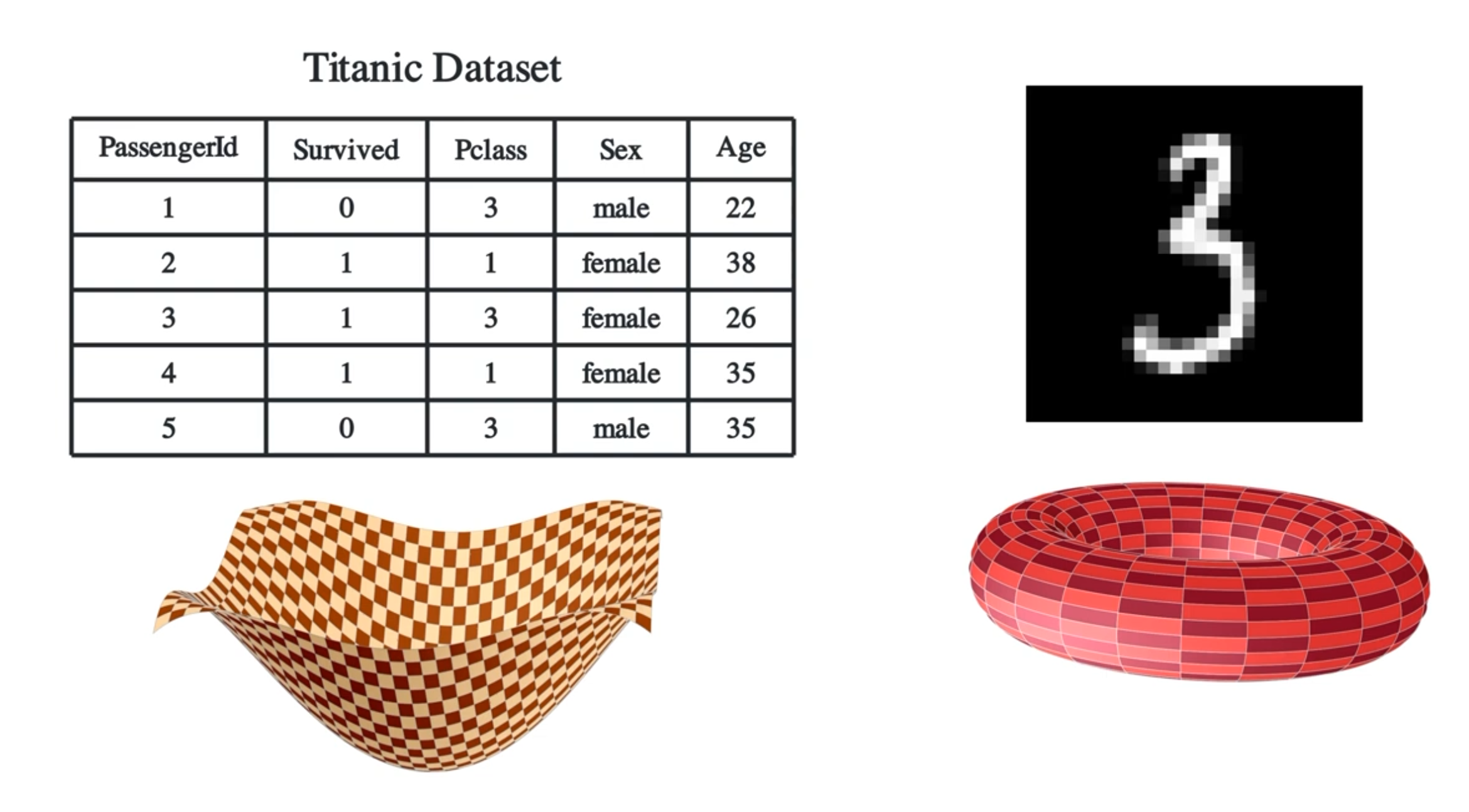
According to the manifold hypothesis, it could be true. The manifold hypothesis says that many high-dimensional data sets that occur in the real world actually lie along low-dimensional manifolds inside that high-dimensional space. To understand what a manifold is, here are a bunch of examples. Examples of one dimensional manifolds lying in a 2 dimensional space include a line or a circle. Two dimensional manifolds are also called surfaces, which include a plane, the outside surface of a sphere, a torus, etc. And just for completeleness, a zero dimensional manifold is a dot.
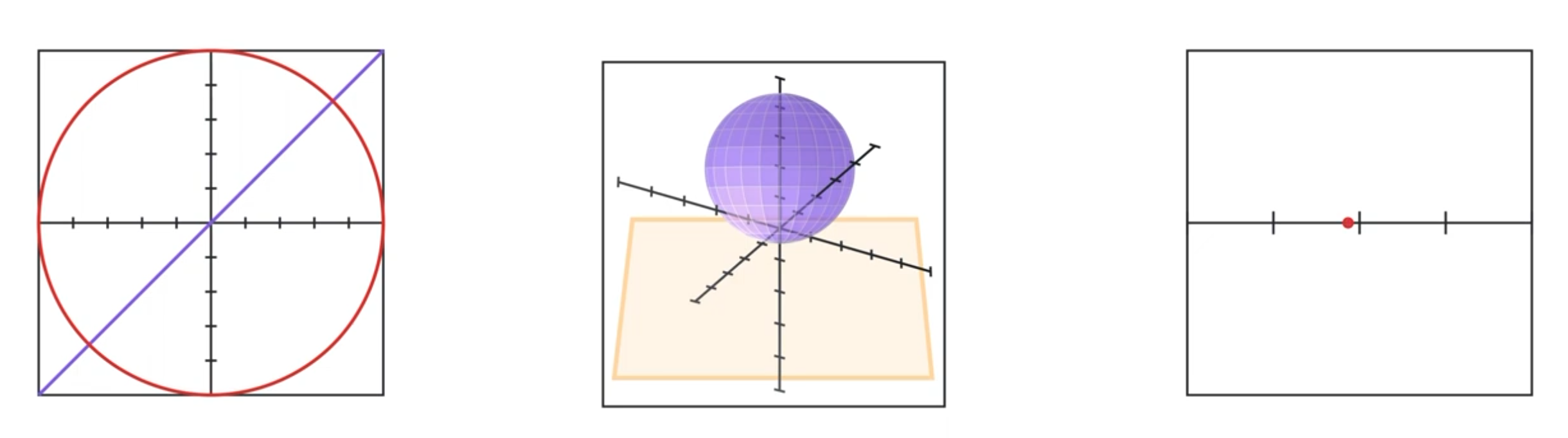
And to repeat, the manifold hypothesis says that real world datasets actually form these manifolds. The goal of the neural network is to then stretch and morph and disentangle these manifolds such that we can finally separate them using hyperplanes.
I think a good way to end this video is to try to show this concept in a real world dataset. Here, I’ll try to visualize what a regular neural network would do on the MNIST dataset, which is a collection of 28 by 28 grayscale images of handwritten digits.
I’ll use this very simple classic neural network, but I won’t bottleneck it to only 2 or 3 units per neurons per layer.
import torch
from torch import nn

class MnistClassifier(nn.Module):
    def __init__(self):
        super(MnistClassifier, self).__init__()
        # fully connected linear layers (FC)
        self.fc1 = nn.Linear(784, 128)
        self.fc2 = nn.Linear(128, 64)
        self.fc3 = nn.Linear(64, 10) # output is 10 dimensions because there are 10 different digits

    def forward(self, x)
        x = torch.tanh(self.fc1(x))
        x = torch.tanh(self.fc2(x))
        return self.fc3(x)
I’ll instead perform PCA on each layer’s output to reduce the dimensions to 3. You don’t need to understand PCA, but it basically linearly projects the data to a lower dimension such that it maintains the maximum amount of variability or structure.

As you can see, by the final layers, the network already found a way to morph the space in such a way as to position the digits into their own clusters.
We can also see how digits that are somewhat similar are closer to one another, which makes sense. In the very high dimensional space where mnist digits lie, digits that are similar to one another should lie close to one another. And when our neural network tries to separate the digits, it can’t help but place similar digits closer to one another.
Neural networks are really not that well understood theoretically, but it can still sometimes be useful to think about how and why this blackbox we call a neural network actually works. I hope this blog post helped at least shine some light inside this black box we call a neural network.